Introduction
Uplift models predict the incremental effect of a treatment on the outcome of an individual. In other words, they answer the causal question of how an individual’s behavior will change if we give him/her a specific treatment. At Wayfair, we build uplift models to inform us of whom to target and how much to bid for the display ads we use in display remarketing. To learn more about this specific business use case, check out Wayfair Data Science Manager Jen Wang’s blog post. Many different researchers have developed methods for modeling uplift; after much exploration, our team has identified uplift decision tree as the winner in most of the backtestings and live A/B tests thus far. In this blog post, we will provide an in-depth description of the uplift decision tree approach, which directly optimizes for uplift.
Overview of Different Uplift Modeling Techniques
Uplift models involve causal inference in the sense that they allow us to know how much an individual’s behavior would have changed had we given him/her treatment. This kind of prediction is counterfactual in nature. For a causal inference problem, we face the inherent challenge of not having a definite response variable for training, since we can only observe the outcome of a specific treatment, or lack thereof, for an individual, e.g. we cannot simultaneous show and not show a customer a display ad and measure the lift.
To solve the problem above, uplift models rely heavily on randomized experiments to estimate the conditional average treatment effect. i.e. given an individual’s features, the expected value of the change in outcome. Researchers have come up with two general approaches to uplift modeling: the meta-learner approach and the direct uplift estimation approach.
The meta-learner approach essentially reformulates the uplift problem into a different kind of problem—or set of problems—and uses existing machine learning models to solve these “translated” problems. Two of the most widely used meta-learner approaches are the two-model approach and the transformed outcome approach. The two-model approach builds two separate predictive models, one to model P(Outcome|Treatment), and the other to model P(Outcome|No Treatment). To obtain the uplift of an individual, we use both models to predict the two probabilities separately and take the difference. This approach is easy to implement, yet it usually fails to capture the weaker uplift signal because building two models increases the noise of the predictions (Radcliffe & Surry, 2011). The transformed outcome approach, as the name suggests, constructs a new target variable from the initial treatment label and outcome label (Athey and Imbens, 2016). Then any conventional machine learning model such as XGBoost can be used to predict the transformed outcome. It can be proved that the expected value of the transformed outcome is equal to the true uplift, and the learned model should be able to predict the uplift. For more details of this approach, you can refer to this Wayfair blog post by Robert Yi and Will Frost who implemented this approach in their pylift package. When the uplift signal is strong, this approach in general has backtesting performance on par with the direct uplift estimation approach discussed below.
The direct uplift estimation approach modifies existing machine learning algorithms to directly optimize for uplift. It is the approach used in uplift random forest, which, as its name implies, is an ensemble of uplift decision trees. We will discuss the uplift decision tree approach in more detail in the following section.
Deep Dive into the Theory behind the Uplift Decision Tree
Several uplift decision tree algorithms exist, each with a different splitting criterion; here, we will discuss those that use the information theoretical splitting criteria presented in “Uplift Modeling in Direct Marketing” (2012) by Piotr Rzepakowski and Szymon Jaroszewicz.
In the case of a single treatment uplift decision tree, each node will contain two separate outcome class distributions, one for the treatment group and one for the control group. Equivalent to maximizing uplift, we want to make the two distributions as far away from each other as possible as we traverse down the tree. The Kullback-Leibler Divergence and squared Euclidean Distance are two measures of the divergence between distributions used in information theory (Eq. 1). The subscript “i” denotes each outcome class, and p_i and q_i are the probabilities of that outcome class i in the treatment and control group, respectively.

Equation 1: Kullback-Leibler Divergence between Two Distributions (top). Squared Euclidean Distance between Two Distributions (bottom).
For a given node in the tree to be split, we can calculate the divergence of the outcome distributions in that node by using one of the two divergence measures above. After a test, A, that splits a tree node into children nodes, we can similarly measure the conditional divergence of the outcome class distributions conditioned on the test A (Eq. 2). In this equation, “a” stands for each of the children nodes; “N” stands for the total number of instances in the parent node; “N(a)” stands for the number of instances in the child node “a”; “D” is the divergence measure. “P^T(Y)” and “P^C(Y)” are the outcome class distributions, and their “|a” variants are the child node a’s outcome class distributions.

Equation 2: Conditional Divergence for a Given Test
For the best split, we want to maximize the gain of the divergence between the outcome class distributions between treatment and control. In other words, we want to maximize Eq. 3. The first term is the conditional divergence referred to above, and the second term is the parent node’s outcome class distribution divergence.

Equation 3: Gain in Class Distribution Divergence for a Given Test
Too many equations? Don’t worry. We have an example below to make it more concrete.
A Toy Example to Help Explain the Theory
To better illustrate how the uplift decision tree splits its nodes by maximizing the gain in the divergence between the treatment and holdout class distributions, we present the following example (see Fig. 1). Imagine we have a total of 8 data points in a given tree node, with 4 instances in the treatment group and 4 instances in the holdout. 3 out of the 4 customers in the treatment group converted, and 2 out of the 4 customers in the holdout group converted. We want to find a way to split this node such that the gain in Eq. 3 is maximized.

Figure 1. An example of a decision tree node being split by maximizing the distributional divergence present in the resulting children nodes. A green circle indicates the customer converted, and a red circle indicates the customer did not convert. The customers in the box labeled “T” are in the treatment group, those in the box labeled “C” are in the control group.
In theory, the uplift decision tree’s splitting criterion is compatible with multiway splits. But in practical implementation, binary splits—where a split will only produce two children nodes—are more common, as is shown in this example. We claim that the split shown in Fig. 1 is the optimal split we are looking for. To prove it, let’s work out the math. For simplicity of calculation, we pick the squared Euclidean distance as the divergence measurement.
First, we calculate the divergence of the class distributions in the parent node:

This is simply the squared Euclidean distance of conversion rate between the treatment group and holdout group ((0.75-0.5)2) plus the squared Euclidean distance of non-conversion rate difference between the two classes ((0.25-0.5)2). Similarly, we can calculate the class distribution divergences for the two children nodes. For the left node we have (1-0)2+(0-1)2=2. For the right node we have (0-1)2+(1-0)2=2.
To normalize the relative influence of the two children nodes on the improvement of the divergence after splitting, we calculate the conditional divergence shown in Eq.2:

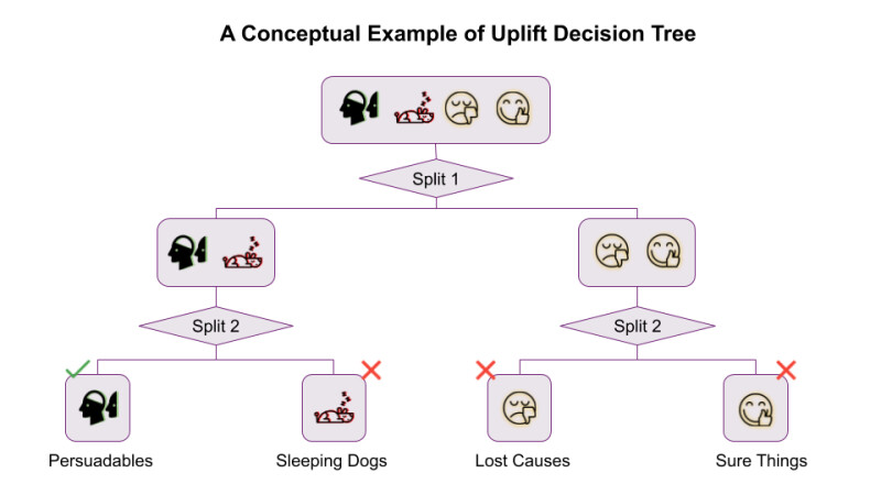
Therefore, the gain in class distribution divergence is 2-0.125=1.875 by Eq. 3; this is the maximum value the gain can take, because the squared Euclidean distances of the two children are maximized (both equal to 2) when the divergence of the two class distributions are the greatest. To speak in more concrete language, the left child node now purely contains the persuadables, because everyone in treatment converted, and everyone in the holdout did not convert. The right child node is just the opposite, and within it contains the do-not-disturbs (or “sleeping dogs”), who generate negative value when they receive treatment.
During model training, this optimal split will be found by iterating through different splits at different values of the available features, calculating the gain for each scenario and picking the split with the highest gain.
Addressing Potential Suboptimal Splits
That wasn’t so difficult to follow, right? Well, there is more to the story. We need to address two potential problems that can arise from the splitting scheme presented above: first, an uneven treatment/control split; second, the tendency for the algorithm to select splits with a large number of children nodes. An uneven treatment/control split occurs when the algorithm puts most—if not all—of the treatment instances in one subtree, and little to no control class in that subtree. This means the feature used for splitting is highly correlated with the treatment label and thus violates the unconfoundedness assumption essential to uplift modeling. Moreover, such a split will make further splits more difficult, because every leaf node has to contain enough treatment and control instances. The second problem, selecting splits with a large number of children nodes, can be an issue because such splits tend to have higher gains when applied to the training data, but extrapolate poorly to the test data, resulting in overfitting.
The normalization factors shown below are designed to correct the aforementioned biases. In this instance, as with the two splitting criterion variants, we have two types of normalization values, one for KL divergence, and the other for Euclidean distance.

Equation 4: Normalization Value for Splitting Based on KL Divergence

Equation 5: Normalization Value for Splitting Based on Euclidean Distance
Since the two penalty terms are quite similar, here we will only discuss the case for Euclidean distance. The first term prevents an uneven treatment/control split. The first part of the first term is the Gini impurity of the class proportions in the parent node; it will be close to zero when there is a large treatment/control imbalance. This is because if there is already a large treatment/control imbalance present in the parent node, then it is not fair to penalize further the resulting children nodes’ imbalances. The second part of the first term is the squared Euclidean distance between the treatment proportion and the holdout proportion in all the children nodes. This value will be minimized only when the two proportions are equal in all the children nodes.
The next two terms penalize tests with large number of children nodes, similar to how the classic decision tree algorithm deals with the same problem. The Gini impurity increases when the number of children nodes after the split increases. For example, when it is an even binary split, we have 1-0.52 -0.52 =0.5, when it is an even four way split, then we have 1-4*0.252=0.75. The final ½ term is present to prevent favoring a split that has a small gain in uplift but is inflated by dividing a small normalization factor.
Future Directions
Although the uplift random forest implementation we use (created by Paulius Šarka) has produced exceptional results in live campaign targeting, we believe we can make further contributions and improvements to the package as we strive to make constant advancement to our modeling techniques through rapid iterations at Wayfair. Below is a list of opportunity areas we have identified that can either boost the performance of the current implementation or expand the use case of our models.
- Multiway split: Although the theoretical formulation accommodates multiway splits when building the tree, the current implementation we use only supports binary splits. Since any multiway split can be achieved by a series of binary splits, from the perspective of model performance there is little gain from implementing this feature. However, if we have a large number of nominal features, multiway splits can significantly reduce the tree depth and improve the interpretability of the model.
- Multi-treatment uplift model: While we only discussed the single treatment case in this blog post, the authors of the uplift decision tree algorithms have separately designed an upgraded version of their algorithms that can handle multi-treatment uplift, where the model will predict the best treatment out of multiple treatments for a given individual (Rzepakowski and Jaroszewicz, 2012). By incorporating this modified algorithm into the code, we will be able to answer important questions such as: which ad creative is most relevant and helpful for our customers? Or, which marketing channel is best suited to reach out to a customer?
- Contextual Treatment Selection Algorithm: This is yet another uplift decision tree algorithm invented by Zhao et al. It directly optimizes for an evaluation metric called expected response which is an unbiased measurement of what the outcome will be given we follow the treatment strategy produced by the model (Zhao and Fang and Simchi-Levi, 2017). This approach has demonstrated impressive backtesting results surpassing that of uplift random forest according to the paper. We are planning to incorporate their new evaluation metric and splitting criterion into the package we use. This initiative will enable us to obtain an unbiased estimate of the backtesting performance for multi-treatment uplift models and potentially improve our model performance.
Summary
In this blog post, we have presented different classes of uplift models and discussed the uplift decision tree approach in detail. We also went over the many improvements we are currently scoping out. If you are as fascinated by this topic as we are, please check back for future updates on our latest progress working with uplift models.
References
Athey, S., & Imbens, G. W. (2015). Machine learning methods for estimating heterogeneous causal effects. stat, 1050(5).
Radcliffe NJ, Surry PD. Real-world uplift modelling with significance based uplift trees. White Paper TR-2011-1, Edinburgh, UK: Stochastic Solutions, 2011.
Rzepakowski, Piotr & Jaroszewicz, Szymon. (2012). Decision trees for uplift modeling with single and multiple treatments. Knowledge and Information Systems - KAIS. 32. 10.1007/s10115-011-0434-0.
Rzepakowski, Piotr & Jaroszewicz, Szymon. (2012). Uplift modeling in direct marketing. Journal of Telecommunications and Information Technology. 2012. 43-50.
Zhao, Yan & Fang, Xiao & Simchi-Levi, David. (2017). Uplift Modeling with Multiple Treatments and General Response Types. 10.1137/1.9781611974973.66.
