Speeding up A/B Tests with Delayed Reward Forecasting

Introduction

As a data-driven tech company, Wayfair constantly conducts A/B tests to optimize our marketing campaigns. In many cases, we either wait for a long time (30-60 days or longer) to measure orders and revenue lift (a.k.a., “delayed rewards”), or resort to upper funnel signals (e.g., click-through-rate, add-to-cart rate) in a shorter window to speed up learning. Ideally, we would want to have the best of both approaches, i.e. to learn fast while optimizing for long-term cumulative rewards.

To that end, we developed Demeter, which is the data science platform that uses ML models to forecast longer term KPIs based on customer activity in the short term. It allows us to optimize our decision/action towards longer term KPIs without having to run long term tests. This adds value in traditional A/B testing by reducing the opportunity cost in designing, executing, and monitoring long term tests.

In this blogpost, we will first explain our model framework and methodology for forecasting longer term business KPI. Then we will discuss how to validate the model performance for A/B testing applications. In the end we’ll discuss how to platformize KPI forecasting models for a wide range of applications.

Model Framework

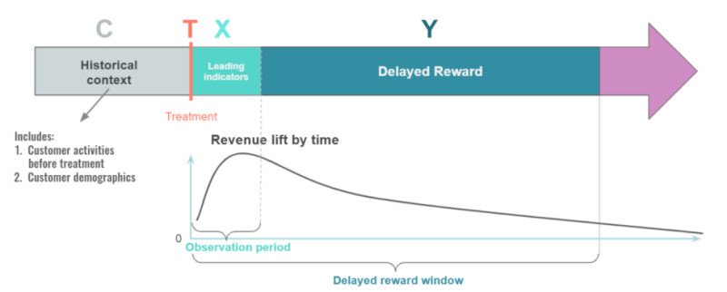
The diagram below (Figure 1) shows the prediction framework for the Demeter platform. Here’s the business problem we want to solve: we launch a new treatment T (e.g., a new marketing ad campaign) at some point in time and would like to know the treatment effect in a longer window (e.g., a few months) without actually waiting that long to measure it. There exist a few different approaches to solve this problem. For example, one can frame this problem as a time series forecasting problem. Most time series forecasting algorithms work best at aggregate level when a rich history of data is available. But in our case, we often need to forecast the delayed reward at individual customer level or small cohort level, based on only a few days’ data. To do that, we build Demeter using a standard ML regression pipeline, where we can use all the information we know about a customer to predict their future reward, which can then be consumed directly or aggregated for applications at cohort level. Specifically, we take the following steps to predict long-term value of an ad treatment:

1. Pull the historical context C for each customer. Historical context is information we know about the customer prior to the ad treatment; 
2. Observe the customer activities shortly after the treatment, which are called leading indicators X, 
3. Predict the delayed reward Y based on the leading indicator X in the observation window and the historical context C. 

Theoretical Foundation

The Demeter modeling framework is based on the surrogate index methodology described in Athey et al. (2019). The authors suggest that one can combine multiple short-term outcomes into a surrogate index which is the predicted value of the long-term outcome of interest given these short-term outcomes. They then prove that one can get an unbiased estimate of the long-term treatment impact from the treatment impact on this index.

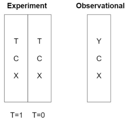
More concretely, Demeter requires two sets of data: one observational dataset and one experimental dataset, as depicted below (Figure 2).

In this diagram, the experimental dataset comes from a A/B test where treatment label T is either 1 (treated) or 0 (not treated). In the observational dataset, however, the treatment label T is not required but the delayed reward measurement Y needs to be available. With this setup, we can lay out the surrogate index approach as the following:

1. Train a predictive model based on the observational dataset to predict the delayed reward as a function of the leading indicators and the historical context.
2. Predict delayed reward Y in the experiment dataset using the mapping learned from the observational dataset.
3. Treat the predictions of the delayed reward as if they are the actual delayed reward. We can take the average predicted delayed reward in the treatment group, and the average predicted delayed reward in the control group, and the difference between the two is the predicted long-term impact of the treatment — even though we don't have actual information on the delayed reward.

It is worth noting that the approach and principle can be applied to general A/B tests where T is the two treatment variations A or B.

Now the question is: what assumptions are needed for this approach to work? Below is a summary of the assumptions, and what we can do to better satisfy these assumptions.

1. Unconfoundedness:

This is the standard requirement in randomized experiments that treatment assignment T is independent of potential outcome X and Y, conditioned on all pre-treatment variables (i.e., historical context) C.
An example of violating this assumption is that customers with high purchase intent (e.g., “I really need a bed for a guest coming next week” vs. “I am just browsing for fun”) are preferentially assigned to group A over group B and the purchase intent is unobserved. In this case, the group difference in delayed reward Y no longer solely represents the true treatment effect - it is confounded by the group difference in purchase propensity. To avoid violations like this, we ensure that our experiment groups are well matched by using either random splits (for large sample sizes) or more precise matching approaches (for small sample sizes).  

2. Surrogacy:

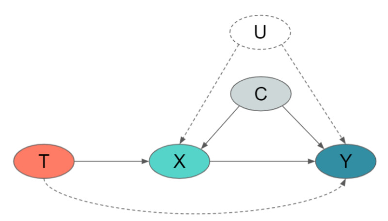
The Surrogacy assumption requires that the delayed reward Y is independent of the treatment T, conditioned on the full set of leading indicators X and the historical context C. To make this abstract statement easier to understand, we represent it in a causal diagram below (Figure 3). In essence, this assumption requires the leading indicators X capture all the causal influence of T on Y. In other words, there should not be any pathway from T to Y that bypasses X, i.e., the dashed line in the bottom of the diagram can not exist.

This is a fairly demanding assumption, and is unlikely to be satisfied if we use just a single short-term metric as the leading indicator, e.g., short term revenue directly reflects business value but may be sparse; clicks are predictive but noisy. Unfortunately, it is hard to test this assumption theoretically. We can run backtest on historical tests to validate this assumption, which we will discuss in more detail in the next section. Intuitively speaking, the assumption becomes more plausible if we include more data in the model. Adding information on browsing time, number of products in category viewed, etc or increasing the observation window length should increase the signal-to-noise ratio. The more short-term metrics we have, the more mechanisms we can account for between treatment T and the delayed reward Y.

The Surrogacy assumption also requires that there are no unobserved pre-experiment characteristics U that affect both the leading indicators X and the delayed reward Y (illustrated in the diagram below). This assumption is also very demanding as we need all of these potential “confounders” between the short-term outcome X and the long-term outcome Y to be observed and included in the historical context C.For example, it is conceivable that whether or not a customer has made the first purchase on Wayfair before the treatment T will have an impact on both the short term and the long term outcomes. A consumer who has purchased from us might be a new homeowner or might have needs in product categories in which we are more competitive. Factors like these can appear in the confounding variable U. Failing to control for confounders like these will bias our estimator. Similar to the above, we can include more pre-experiment characteristics C to reduce the likelihood that an unobserved characteristic U would affect both X and Y.   

3. Comparability:

This requires that the conditional distribution of the delayed reward Y given the leading indicator X is the same in the observational and experimental samples. For example, if we use pre-pandemic data as the observational data to train the model, and apply the model to predict the delayed rewards in a post-pandemic experiment, the prediction will not be very accurate since the mapping from C, X to Y likely changed after the pandemic. To better satisfy this assumption, we use the most recent data available, or data most representative of the current treatment to train the Demeter model.

Model Validation

If these three assumptions are satisfied, then the surrogacy approach above should work and we can predict the long-term impact of our treatment. How do we know if these assumptions hold up in real-world applications?

1. We can use out-of-sample validation to boost our confidence in the surrogacy assumption. For example, if we can show that predicted Y based on the short-term metrics in the first 7 days closely tracks the effect measured in 15, 30, 60 days after the treatment, we would be more confident the assumption will hold up to longer-terms, e.g., 90 days or 120 days. 
2. Practically speaking, we need to validate the modeling approach in backtests for each of the use cases. If the predicted lift closely matches the actual lift, we would be more confident that the assumptions are holding up for that use case. 

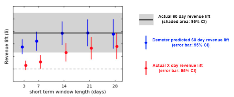
As an example, the plot below (Figure 4) shows the model validation result from a lift study at Wayfair that ran over 60 days (revenue data are masked for illustrative purposes only). We trained the model on campaigns (observational data) prior to the lift study (experiment) using different observation window lengths (3, 7, 14, 21, 28 days) to predict the 60 day lift in revenue per customer after the treatment.

For each short term window length, the gap between the red dot and the black line is the true “delayed reward”, i.e. the revenue impact we would miss if we only read the first X days revenue lift by the ad treatment. In contrast, Demeter captures a portion of the delayed reward as indicated by the vertical distance between the blue and red dots for each X-day period. As early as day 3, Demeter has already captured a significant portion of the delayed reward. In fact, the predicted 60 day revenue lift is already within the confidence interval (CI) of the true 60 day lift while the actual 3-day revenue lift is not even significantly above 0. As we use longer observation windows, the prediction continues to improve and captures a higher percentage of the delayed reward. At day 14, for this particular example, the predicted lift is essentially right on top of the actual lift, while the actual 14-day lift only accounts for less than half the full 60-day lift.The implications from this backtest are two fold: first, using the surrogacy methodology, we can make accurate predictions on the 60-day lift when using an observation window of at least 14 days in this use case. While a good backtesting result cannot completely “prove” the assumptions, it provides us sufficient confidence in the surrogate index methodology for practical purposes, especially when a theoretical validation of the assumptions in real life use cases is very difficult, if not impossible. Second, for this use case, Demeter prediction allows us to make business decisions much earlier than the 60-day test duration.

We have done similar validation in multiple A/B tests in different marketing channels. The results are similar to the example above, although different channels may require different short term window sizes to converge.

Demeter as a Platform

In general, there’s quite a wide array of unique forecasting problems related to mapping the relationship between some short-term measurable engagement metrics to some longer-term business outcomes. While there’s a lot of variety in nuances of the specific forecasting needs across various channels, treatments, and funnel depths, there are a core set of fundamental dimensions by which these needs vary and we believe a well-designed ML platform should be able to handle most applications under a single technology. For example, we might change the short term observation window from “first 3 days” to “first 7 days”, or change the prediction unit from “Customer-level” to “visit-level” in another use case. Our long-term goal is for the platform to be able to support any combination of parameters in these dimensions.

To sum up, in this post, we introduced Demeter - our inhouse delayed reward forecasting platform at Wayfair. We talked about the theoretical foundations of the “delayed reward” forecasting problem and explained its use cases in marketing A/B tests. Demeter can also be used as the “reward generation” component of an online ML system (e.g., Waylift, our in-house marketing decision engine, described in a previous post). For example, Demeter could forecast business KPIs (e.g. 60-day revenue) from short-term upper-funnel metrics (e.g. clicks, product page views), contingent on assumptions being respected. This delayed reward forecast would enable the online ML system to make faster decisions while still optimizing towards longer term KPIs, and to make tradeoffs between transactional goals and business growth strategy, e.g., “sell more products in existing categories now” vs. “strategically add new categories of product in the catalog”. We will discuss more about the RL use case in a future post. Stay tuned!