Introduction
Explainable Artificial Intelligence (XAI) is an emerging field within Machine Learning (ML). There has been considerable advances in the state of the art in recent years.
Machine learning models often need to be audited for bias and unfairness. Effectively interpreting the decision of an algorithm is an integral part of this process. Model explanation is also highly relevant for cases where ML models need to operate with a human-in-the-loop.
In this blog post we are going to focus on Fraud detection. One particular use case is 'Payments Fraud' whereby criminals attempt to use stolen credit cards to purchase items on Wayfair. We are going to treat this as a supervised, binary classification problem where orders are either fraudulent or not.
In practice, we found that separating orders in three buckets provides better results. A small percentage of orders for which the model is not sure are then sent to specialized human reviewers who manually investigates and evaluates the riskiness of the order. In these situations, a model's ability to explain its prediction becomes critical for supporting human reviewers' forensic process.

In this blog post, we will provide an overview of explanation / interpretation methods for supervised machine learning models and provide a deep dive into their application to Fraud Detection. We will discuss different explanation methods such as Permutation importance, Lime and SHAP and see how they differ in a specific application to a toy dataset of fraudulent orders.
Overview of different methods
Machine learning (ML) algorithms tend to be high-dimensional, non-linear and complex. For example, neural networks often contain millions or even billions of parameters. Understanding why an ML algorithm made a certain decision can be a challenging task. Many practitioners treat complex algorithms as a black-box. The field of interpretability for ML aims to alleviate that task and open up that black-box.
Local and global interpretations
First of all, we need to distinguish between two types of explainability: local (or individual) explanations and global (or general) explanations. Global explanations aim to understand the model and unveil the importance of input features over all data points. Local explanations, on the other hand, explain why an ML algorithm made a certain decision for a single data point. For fraud detection, we are generally more interested in local explanations because those are the ones manual reviewers will use to base their decisions on.
Interpretable models
The easiest way to obtain explanations is to use simple models. Let's consider linear or logistic regression, for example. The predictions of these algorithms are modeled as a weighted sum of the input. We can simply look at the weights associated with each input feature and interpret their importance based on the magnitude of the weights. Another example of interpretable models is decision trees or random forests. Obtaining a local explanation for a decision tree is simple: starting from the root node we go down the tree. The conditions at each node can serve as an explanation for the final prediction. We are going to see an example in later sections of this blog post. For a global explanation, we can measure how much each node reduces the variance (or Gini impurity) of the data times the probability of reaching that node. K-nearest neighbors is another algorithm that naturally provides local explanations. We can explain a sample of interest, by analyzing its k-most similar neighbors.
The main disadvantage of these algorithms is that they are not very accurate for most practical problems. There seems to be an inherent tradeoff between predictive performance and effective interpretation of results. In the following sections, we will explore model-agnostic methods used for complex algorithms such as neural networks.
Permutation importance
Permutation-based explanations are straightforward. First, we measure the baseline reference score for a sample or collection of samples. This score can be the error or prediction probability for the correct class of an ML model. Then, we perturb the input features and see how that affects the output of the model. Some perturbations will lead to a greater loss in accuracy than others. We can rank features based on the magnitude of the error their perturbation caused.
Shuffling the values of "important" features should cause a significant drop in performance. If the model error remains unchanged after we perturb a feature, we can consider this feature "unimportant".
One disadvantage of permutation importance is that correlated features can have decreased importance. Say we use price_of_order and most_expensive_product_price as inputs to a fraud detection algorithm. Those features will be highly correlated and it is likely that removing one of them will not have a significant impact on model performance. A simple permutation algorithm will not capture the true importance of these features if it permutes one feature at a time.
Lime
Lime [2] is short for Local Interpretable Model-Agnostic Explanations. This approach only explains individual predictions. The idea is the following: we want to understand why a black-box classifier f made a certain prediction for data point x. Lime takes x and generates a new dataset containing many different variations (or perturbations) of x. These artificial samples are denoted as zi , i {1,...,N}. Black-box predictions f (zi) are obtained. Lime then trains a new, simpler, interpretable model with zi as inputs and f (zi) as a target. Each artificial sample is weighed by how close it is to the original data point x at which we evaluate our model. We already saw examples of interpretable models in the section above. The final step is to explain x by looking at the weights of the interpretable model (also called a "local surrogate" model). The algorithm from the original Lime paper [2] can be found below.
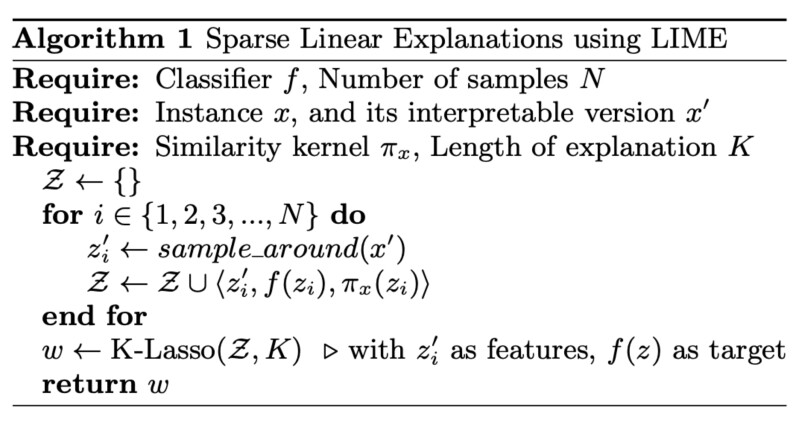
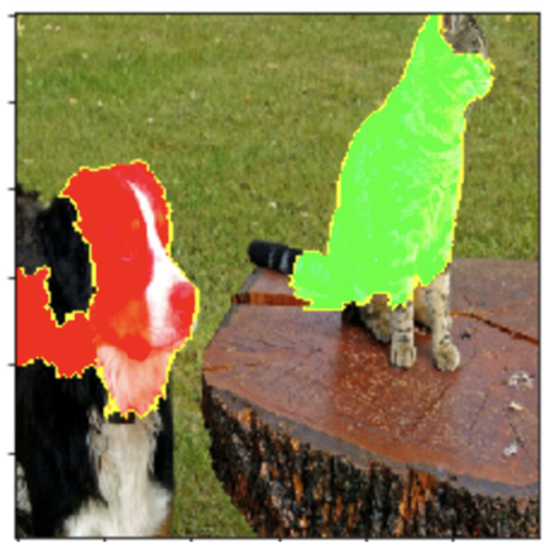
An example local explanation applied to images can be found in Figure 2. We can also train a "global surrogate" model to obtain global predictions. The idea is very similar: we train a simple model to approximate the predictions of a black-box model. The key difference is that we can also use a number of different data points for training.
SHAP
In coalitional game theory, Shapley value [3] is a way of fairly distributing gains and losses to actors working in a coalition. This concept is mainly used when the contributions of actors are unequal. For the case of Machine Learning, we can treat the feature values of a sample as "actors" and the final prediction probability as the "gains and losses".
Say we want to compute the importance of feature i via Shapley values. First, we need to obtain all possible coalitions of features which need to be evaluated with and without feature i. In practice, this is often very expensive as the number of features grows. In these cases, Shapley values are approximated by randomly sampling possible coalitions.
SHAP [4] stands for SHapley Additive exPlanations. Kernel SHAP is a model agnostic implementation of SHAP. This method combines the theory of Shapley values with local surrogate models such as Lime. If we need to evaluate the prediction of model f at instance x, we would sample Kcoalitions (or K variations of x ). Then we would obtain the black-box model predictions for those coalitions and fit a weighted linear model to this data. This process seems very similar to Lime.
There are a few key differences between Kernel SHAP and Lime, however. For example, the weighing of instances is conceptually different. Lime calculates similarity via the radial basis function kernel. SHAP weighs instances based on the coalition Shapley value estimation. This is achieved by the SHAP kernel described in [4].
SHAP also has a fast implementation on tree-based models [5]. This makes it possible to also use SHAP for faster global explanations. SHAP shows more consistent local explanations compared to Lime. Advantages and disadvantages of both methods are well-described in [1].
Toy example
In this section, we will illustrate how different explanations work in practice. We artificially generated a toy dataset of 1000 orders. Suppose that for each order we have the following information:
- Index: Unique identifier of the order.
- AgeOfAccountDays: How many days have passed since account creation.
- BillingShippingCityMatch: Binary feature indicating if the billing address city matches with the shipping address city.
- HasPreviousOrder: Binary indicator showing if the customer has a previous order.
- 2FA: Binary indicator showing if the customer used 2-Factor-Authentication.
- HatColor: Hat color of the customer.
- ShoeSize: Customer shoe size.
- FavouriteCoffee: Favourite coffee of the customer.
We labeled the orders with no 2FA, no previous order history, no billing/shipping city match, and an age of account lower than 20 days as 'Fraud' for the sake of the experiment. You might notice that the last three features we used are redundant and do not affect the Fraud label. The structure of the dataset is shown in Figure 3. A good explanation method should be able to pick up this information and assign an importance value equal to 0 to these features.

We trained a decision tree classifier to solve this binary classification problem using the sk-learn implementation of this algorithm. After training, the model achieved 100% accuracy on the test set. What we are more interested in, however, is the feature importance obtained from this example model.
Default Decision Tree Explanation
First, we obtain the default feature importance values provided by sk-learn. Global feature importance is defined as the overall improvement in the quality of the model prediction brought by that feature. In Figure 4, we can see that, although in theory the top-4 features are equally important, the default explanation assigns very different importance scores from one feature to another. Redundant features were correctly assigned 0 importance.
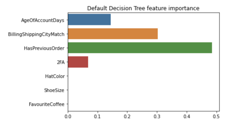
To understand why this is the case we need to look at the gini index for each node of the decision tree illustrated on Figure 5.
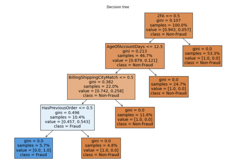
Furthermore, if we are interested in local explanations, we can simply go down the decision tree and follow the node logic. For example, let's explain the ML decision for order with order_id=10000 shown on Figure 3. 2FA is equal to 0 but AgeOfAccountDays is equal to 652 hence the order is classified as Non-Fraud because the customer account was created almost 2 years ago.
Permutation Explanation
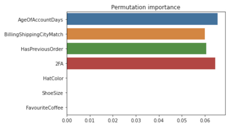
Let's now have a look at the permutation feature importance, implemented by sk-learn, for this Decision Tree Classifier. In Figure 6, we show the global feature importance of our classifier. We can immediately spot that importance is almost equally distributed between the four main features as opposed to the default Gini importance distribution where these features were not 'equally important'.
The sk-learn permutation importance implementation does not work for local explanations, however. In the next section we are going to see examples of local explanations obtained with Lime as well as SHAP examples for both global and local explanations.
Lime explanations
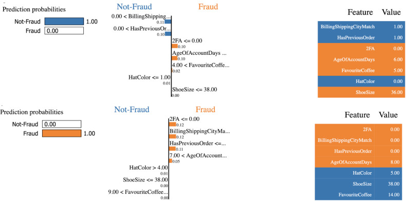
We obtained two local Lime explanations: one for a fraudulent order and one for a safe order. The explanations are shown on Figure 7. We used the lime tabular explainer for this purpose. Input features can have a positive impact (they contribute to the order being classified as 'Fraud') or negative impact (they contribute to the order being classified as 'Non-Fraud'). We can see that, in some cases, certain features can have a positive impact on the 'Fraud' label (orange) while in other cases they have a negative impact on the 'Fraud' label (blue). For the 'Fraudulent' case, the four important features contribute positively to the prediction label, hence the order is correctly classified as 'Fraud'.
An interesting observation is that FavouriteCoffee and HatColor have a non-zero importance for the non-fraudulent example while HatColor has a non-zero importance for the fraudulent example.
SHAP explanations
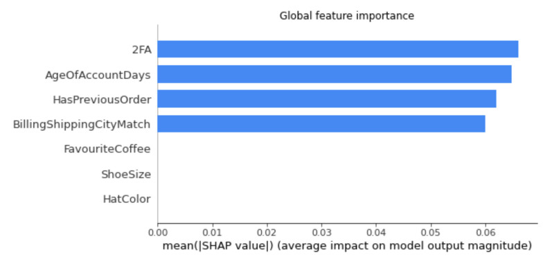
We now turn to SHAP explanations. To this end, we can use the TreeExplainer provided by the shap open source library to interpret our decision tree. TreeExplainer [5] is a high-speed implementation of the SHAP method for trees. This makes it possible to also use SHAP for faster global explanations. An example global SHAP explanation is shown on Figure 8.
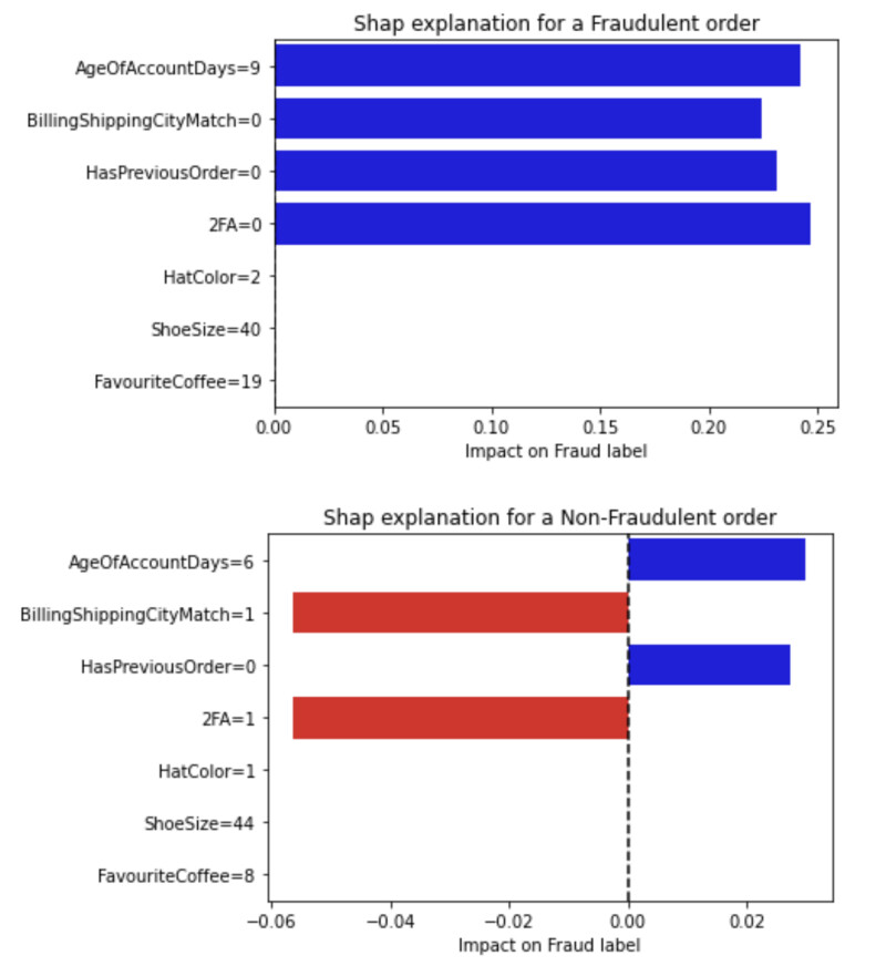
With SHAP we can also obtain local explanations relatively quickly. Again, importance is similar among important features. Unlike Lime, SHAP correctly assigned 0 importance to redundant features. We can see examples of individual explanations both for fraudulent and non-fraudulent orders on Figure 9.
Summary
Explanation methods are essential for trust and transparency of ML decisions. There has been a great amount of work done in the field of explainability in recent years. In this blog post, we cover some basic explainability approaches, such as permutation importance, as well as some more advanced, commonly-used methods such as Lime and SHAP. We applied these explainability methods on a simple decision tree classifier trained on an artificial fraud dataset.
Ultimately, there is no perfect explanation method. Each approach has its advantages and disadvantages. Ideally, an ensemble of explanation methods would yield most trustworthy results. For the readers who want to get a comprehensive overview into the field, I strongly recommend reading "Interpretable machine learning" by Christoph Molnar [1].
You can find a colab notebook in which we artificially created this dataset, trained a model and obtained multiple different explanations
HERE.
References
[1] Molnar, Christoph. "Interpretable machine learning. A Guide for Making Black Box Models Explainable", 2019. https://christophm.github.io/interpretable-ml-book/.
[2] Ribeiro, Marco Tulio, Sameer Singh, and Carlos Guestrin. "Why should I trust you?: Explaining the predictions of any classifier." Proceedings of the 22nd ACM SIGKDD international conference on knowledge discovery and data mining. ACM (2016).
[3] Shapley, Lloyd S. "A value for n-person games." Contributions to the Theory of Games 2.28 (1953): 307-317.
[4] Lundberg, Scott M., and Su-In Lee. "A unified approach to interpreting model predictions." Advances in Neural Information Processing Systems. 2017.
[5] Lundberg, S.M., Erion, G., Chen, H. et al. "From local explanations to global understanding with explainable AI for trees." Nat Mach Intell 2, 56–67 (2020).
Open source libraries
SK-learn: https://github.com/scikit-learn/scikit-learn
Lime: https://github.com/marcotcr/lime
SHAP: https://github.com/slundberg/shap

